
omnichrome.py█
Omnichrome is a project I’ve been working on for almost as long as I’ve been able to code. I use it as a practice project to make sure I stay in form when I’m not doing much coding at work or school.
What does it do?
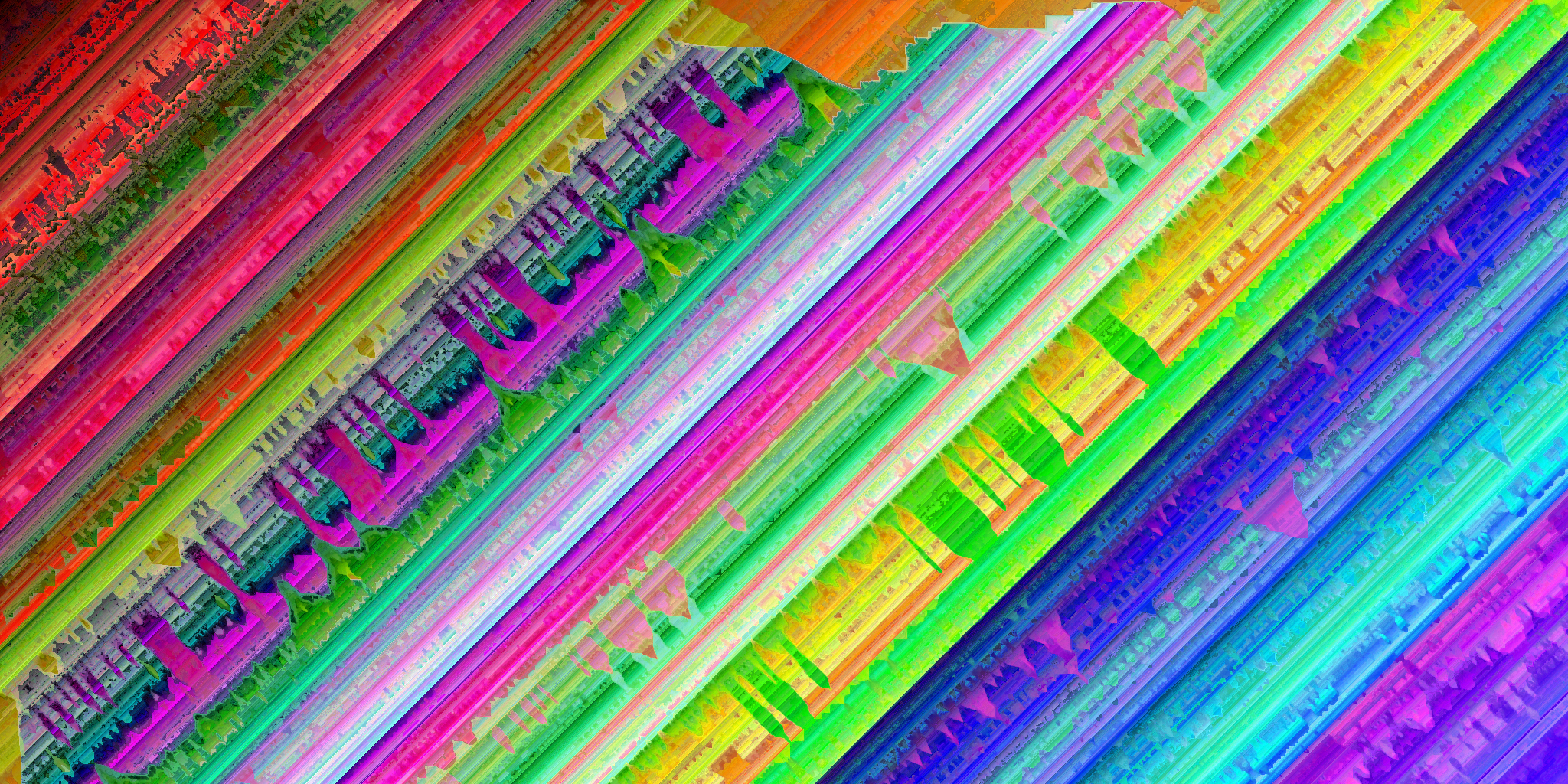
Omnichrome makes images.
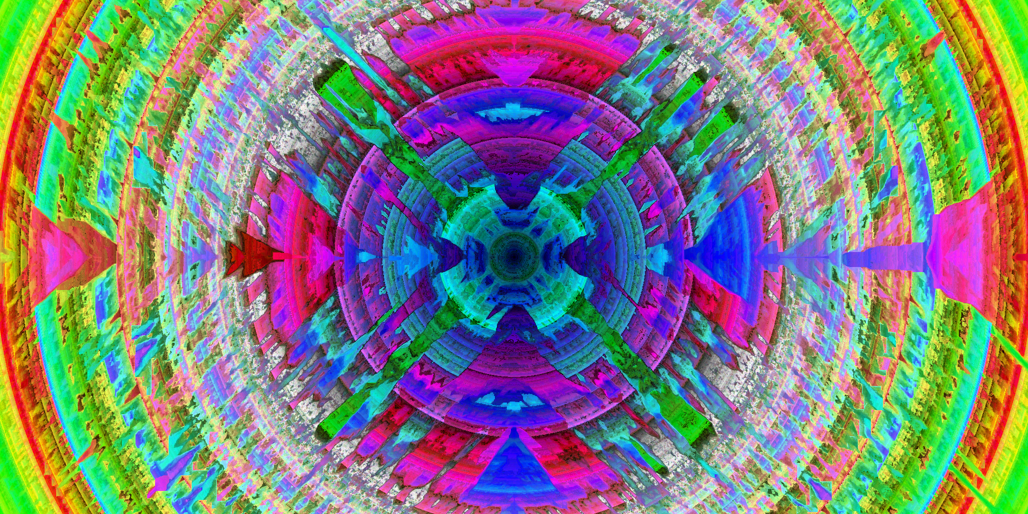
It makes pretty, colorful, fractal-esque images.
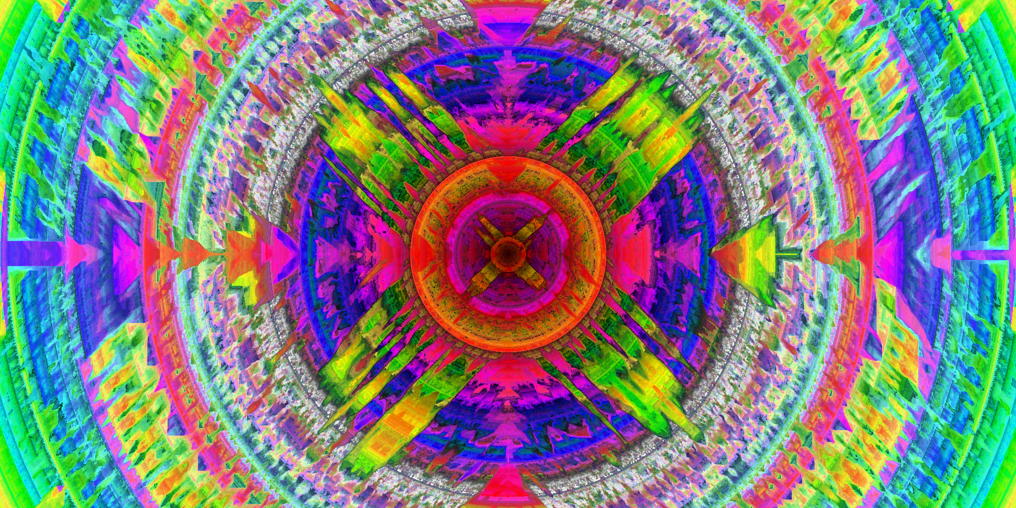
Every pixel in the images is unique; every possible 7-bit color is there exactly once.
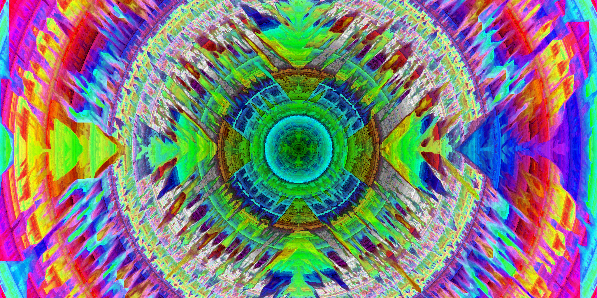
These images are produced by the current iteration, which is 5th or 6th total version of the program.
The original inspiration was a post on codegolf.stackexchange that challenged competitors to create images with every color. They link to allrgb.com; who knows where the original idea came from.
I wrote my first version in middle school. I used a language called processing, which is really just Java with a nice graphics interface. I only have one sample that survived from that version:
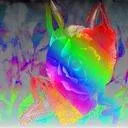
Honestly, I still think it kinda looks good but realistically there’s no way it’s actually omnichromatic (meaning a unique and spanning set of pixels).
The newest version is a lot more complex than that original version. In a sentence, it uses a K-D tree to iteratively place the nearest unused pixel in color to the neighbors moving outward from the center. At a high level that isn’t too complicated, but the details get pretty messy pretty quickly.
How to build an Omnichrome
Step One: Make a stochastic 3D Voronoi partition of the entire colorspace
Stochastic 3D Voronoi Partition. What?
A Voronoi pattern is made by selecting a bunch of points on the plane, then coloring the plane based on the nearest point. Wikipedia has a nice example:

We’re doing the same thing, but we’re grouping colorspace instead of normal euclidian space. However, since humans have three differently colored cones in our eyes, we need three dimensions in our colorspace, so we get more of a Voronoi Cube than a Voronoi Diagram.
That’s not so hard. We’re randomly (stochastically) selecting a bunch of colors, and grouping the rest of the colorspace by which color is closest (Voronoi partitioning). Stochastic 3D Voronoi Partitioning. Neat.
Step Two: The K-D Tree
Use the Voronoi Partitions to build a K-D Tree
A K-D Tree is a binary tree used to partition spacial data instead of just numerical data. It works in some K number of dimensions instead of just one; a binary tree is a special case of a K-D tree where K=1. Normally, a K-D tree works somewhat differently than in our case. The Voronoi partioning gives much more asthetically pleasing results, but it isn’t a part of the normal process.
For our case, we just use each group from the previous step (the Voronoi partitions) as a single branch of the tree. A normal K-D Tree has only two branches per step - we can have any number (although only one branch would be a pretty sad tree).
The ‘key’ for each branch is just the point that corresponded to that group. Later, when we want to search through the tree, we just compare the color we’re searching to each branch’s initial color.
Now, we just need to iterate the process: each sub-group from the original Voronoi partition is broken into a pattern of even more Voronoi partitions. Continue until each partition only has one pixel.
Efficiently partitioning the whole space is a can of worms I don’t want to get into right now, but a push in the right direction would be to imagine each selected color as a heavy mass on a rubber sheet, and to imagine the other colors in the space as particles sliding down towards that color.
Step Three: Search the Tree
Starting in the middle of the image, place each pixel from the tree
This part is easier. Since we already have the tree, it’s now pretty easy to search it for colors. All we have to do is this:
- Pick a pixel to place; start at the middle, and spiral outward to the edges.
- Average the neighboring pixels; search the K-D Tree for the nearest color to this average.
- Pop that color out of the tree; place it at this pixel.
- Return to step 1 until we’re out of pixels.
And that’s it. Tadaa! You’ve made an omnichromic (omnichromatic?) picture!
Step Four: Tune the result
Lots of parameters can be changed and tuned here to make better looking outputs. For example, when making the Voronoi partitions, there’s not really a good reason to use the normal Euclidian metric. I found the best results come from using a skewed metric which uses Hue, Saturation, and Value as the basis, treats Hue as circular, and weights distances in Hue stronger when Saturation and Value are higher.
There’s also no reason you have to start in the middle and spiral out:
I personally think the circular ones are best, but to each their own. Someday I’ll probably write another version, but this is the project as it stands.
Thanks for reading.